Линейная регрессия
Введение
Линейная регрессия это алгоритм машинного обучения с учителем. Иными словами - алгоритму для обучения необходимо указать как входные данные так и заранее подготовленные выходные данные. Всё месте это называется обучающей выборкой. Линейная регрессия может предсказать только одно значение из бесконечно большого диапазона значений, например температуру, скорость движения спутника, и так далее.
Линейная регрессия может быть двух видов:
Простая регрессия
Простая линейная регрессия в своей основе содержит простейшую линейную формулу:
Где \(m\) и \(b\) это значения, которые необходимо подобрать алгоритму для достижения наилучшей точности в своих предсказаниях. Значение \(x\) представляет собой входные данные и \(y\) представляет собой выходные данные.
Множественная регрессия
Более сложная форма линейной регрессии с несколькими переменными. Значения \(w\) являются коэффициентами (ещё их называют «весами» - англ. weight), а \(x_1\), \(x_2\), \(x_3\), … входными значениями. В данном случае алгоритм подбирает значения \(w\).
Простая регрессия
Давайте представим что у нас есть следующая таблица с колонками:
| Компания | Затраты на рекламу | Продажи |
| Amazon | 37.8 | 22.1 |
| 39.3 | 10.4 | |
| 45.9 | 18.3 | |
| Apple | 41.3 | 18.5 |
Далее мы обучим линейную модель для предсказания количества продаж в зависимости от потраченных на рекламу денег.
Предсказывание
Наша предсказывающая модель будет выводит приближенное значение продаж в зависимости от затрат на рекламу по простой формуле линейного уравнения:
или в англоязычных терминах:
- Weight
- коэффициент независимой переменной Advertisment. В машинном обучении такие коэффициенты называют весами (weights).
- Advertisment
- независимая переменная. В машинном обучении такие переменные называют признаками (features).
- Bias
- Параметр смещения относительн оси y. В машинном обучении этот параметр также называют bias.
Our algorithm will try to learn the correct values for Weight and Bias. By the end of our training, our equation will approximate the line of best fit.

Code
def predict_sales(radio, weight, bias):
    return weight*radio + bias
Cost function
The prediction function is nice, but for our purposes we don’t really need it. What we need is a cost function so we can start optimizing our weights.
Let’s use MSE (L2) as our cost function. MSE measures the average squared difference between an observation’s actual and predicted values. The output is a single number representing the cost, or score, associated with our current set of weights. Our goal is to minimize MSE to improve the accuracy of our model.
Math
Given our simple linear equation \(y = mx + b\), we can calculate MSE as:
Примечание
- \(N\) is the total number of observations (data points)
- \(\frac{1}{N} \sum_{i=1}^{n}\) is the mean
- \(y_i\) is the actual value of an observation and \(m x_i + b\) is our prediction
Code
def cost_function(radio, sales, weight, bias):
    companies = len(radio)
    total_error = 0.0
    for i in range(companies):
        total_error += (sales[i] - (weight*radio[i] + bias))**2
    return total_error / companies
Gradient descent
To minimize MSE we use Gradient Descent to calculate the gradient of our cost function. [TODO: Slightly longer explanation].
Math
There are two parameters (coefficients) in our cost function we can control: weight \(m\) and bias \(b\). Since we need to consider the impact each one has on the final prediction, we use partial derivatives. To find the partial derivatives, we use the Chain rule. We need the chain rule because \((y - (mx + b))^2\) is really 2 nested functions: the inner function \(y - mx + b\) and the outer function \(x^2\).
Returning to our cost function:
We can calculate the gradient of this cost function as:
Code
To solve for the gradient, we iterate through our data points using our new weight and bias values and take the average of the partial derivatives. The resulting gradient tells us the slope of our cost function at our current position (i.e. weight and bias) and the direction we should update to reduce our cost function (we move in the direction opposite the gradient). The size of our update is controlled by the learning rate.
def update_weights(radio, sales, weight, bias, learning_rate):
    weight_deriv = 0
    bias_deriv = 0
    companies = len(radio)

    for i in range(companies):
        # Calculate partial derivatives
        # -2x(y - (mx + b))
        weight_deriv += -2*radio[i] * (sales[i] - (weight*radio[i] + bias))

        # -2(y - (mx + b))
        bias_deriv += -2*(sales[i] - (weight*radio[i] + bias))

    # We subtract because the derivatives point in direction of steepest ascent
    weight -= (weight_deriv / companies) * learning_rate
    bias -= (bias_deriv / companies) * learning_rate

    return weight, bias
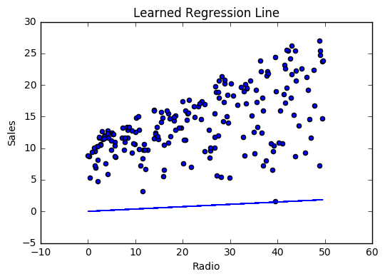
Training
Training a model is the process of iteratively improving your prediction equation by looping through the dataset multiple times, each time updating the weight and bias values in the direction indicated by the slope of the cost function (gradient). Training is complete when we reach an acceptable error threshold, or when subsequent training iterations fail to reduce our cost.
Before training we need to initializing our weights (set default values), set our hyperparameters (learning rate and number of iterations), and prepare to log our progress over each iteration.
Code
def train(radio, sales, weight, bias, learning_rate, iters):
    cost_history = []

    for i in range(iters):
        weight,bias = update_weights(radio, sales, weight, bias, learning_rate)

        #Calculate cost for auditing purposes
        cost = cost_function(features, targets, weights)
        cost_history.append(cost)

        # Log Progress
        if i % 10 == 0:
            print "iter: "+str(i) + " cost: "+str(cost)

    return weight, bias, cost_history
Model evaluation
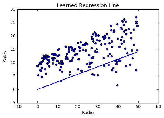
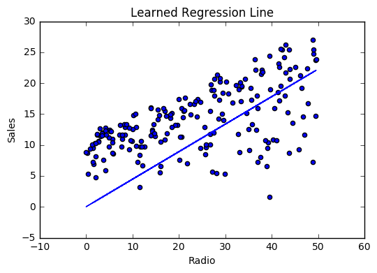
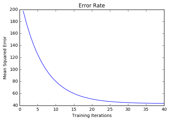
If our model is working, we should see our cost decrease after every iteration.
Logging
iter=1     weight=.03    bias=.0014    cost=197.25
iter=10    weight=.28    bias=.0116    cost=74.65
iter=20    weight=.39    bias=.0177    cost=49.48
iter=30    weight=.44    bias=.0219    cost=44.31
iter=30    weight=.46    bias=.0249    cost=43.28
Visualizing

Cost history
Multivariable regression
Let’s say we are given data on TV, radio, and newspaper advertising spend for a list of companies, and our goal is to predict sales in terms of units sold.
| Company | TV | Radio | News | Units |
| Amazon | 230.1 | 37.8 | 69.1 | 22.1 |
| 44.5 | 39.3 | 23.1 | 10.4 | |
| 17.2 | 45.9 | 34.7 | 18.3 | |
| Apple | 151.5 | 41.3 | 13.2 | 18.5 |
Growing complexity
As the number of features grows, the complexity of our model increases and it becomes increasingly difficult to visualize, or even comprehend, our data.
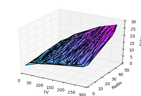
One solution is to break the data apart and compare 1-2 features at a time. In this example we explore how Radio and TV investment impacts Sales.
Normalization
As the number of features grows, calculating gradient takes longer to compute. We can speed this up by «normalizing» our input data to ensure all values are within the same range. This is especially important for datasets with high standard deviations or differences in the ranges of the attributes. Our goal now will be to normalize our features so they are all in the range -1 to 1.
Code
For each feature column {
    #1 Subtract the mean of the column (mean normalization)
    #2 Divide by the range of the column (feature scaling)
}
Our input is a 200 x 3 matrix containing TV, Radio, and Newspaper data. Our output is a normalized matrix of the same shape with all values between -1 and 1.
def normalize(features):
    **
    features     -   (200, 3)
    features.T   -   (3, 200)

    We transpose the input matrix, swapping
    cols and rows to make vector math easier
    **

    for feature in features.T:
        fmean = np.mean(feature)
        frange = np.amax(feature) - np.amin(feature)

        #Vector Subtraction
        feature -= fmean

        #Vector Division
        feature /= frange

    return features
Примечание
Matrix math. Before we continue, it’s important to understand basic Linear Algebra concepts as well as numpy functions like numpy.dot().
Making predictions
Our predict function outputs an estimate of sales given our current weights (coefficients) and a company’s TV, radio, and newspaper spend. Our model will try to identify weight values that most reduce our cost function.
def predict(features, weights):
  **
  features - (200, 3)
  weights - (3, 1)
  predictions - (200,1)
  **
  return np.dot(features,weights)
Initialize weights
W1 = 0.0
W2 = 0.0
W3 = 0.0
weights = np.array([
    [W1],
    [W2],
    [W3]
])
Cost function
Now we need a cost function to audit how our model is performing. The math is the same, except we swap the \(mx + b\) expression for \(W_1 x_1 + W_2 x_2 + W_3 x_3\). We also divide the expression by 2 to make derivative calculations simpler.
def cost_function(features, targets, weights):
    **
    Features:(200,3)
    Targets: (200,1)
    Weights:(3,1)
    Returns 1D matrix of predictions
    **
    N = len(targets)

    predictions = predict(features, weights)

    # Matrix math lets use do this without looping
    sq_error = (predictions - targets)**2

    # Return average squared error among predictions
    return 1.0/(2*N) * sq_error.sum()
Gradient descent
Again using the Chain rule we can compute the gradient–a vector of partial derivatives describing the slope of the cost function for each weight.
def update_weights(features, targets, weights, lr):
    '''
    Features:(200, 3)
    Targets: (200, 1)
    Weights:(3, 1)
    '''
    predictions = predict(features, weights)

    #Extract our features
    x1 = features[:,0]
    x2 = features[:,1]
    x3 = features[:,2]

    # Use matrix cross product (*) to simultaneously
    # calculate the derivative for each weight
    d_w1 = -x1*(targets - predictions)
    d_w2 = -x2*(targets - predictions)
    d_w3 = -x3*(targets - predictions)

    # Multiply the mean derivative by the learning rate
    # and subtract from our weights (remember gradient points in direction of steepest ASCENT)
    weights[0][0] -= (lr * np.mean(d_w1))
    weights[1][0] -= (lr * np.mean(d_w2))
    weights[2][0] -= (lr * np.mean(d_w3))

    return weights
And that’s it! Multivariate linear regression.
Simplifying with matrices
The gradient descent code above has a lot of duplication. Can we improve it somehow? One way to refactor would be to loop through our features and weights–allowing our function handle any number of features. However there is another even better technique: vectorized gradient descent.
Math
We use the same formula as above, but instead of operating on a single feature at a time, we use matrix multiplication to operative on all features and weights simultaneously. We replace the \(x_i\) terms with a single feature matrix \(X\).
Code
X = [
    [x1, x2, x3]
    [x1, x2, x3]
    [x1, x2, x3]
]

targets = [
    [1],
    [2],
    [3]
]

def update_weights_vectorized(X, targets, weights, lr):
    **
    gradient = X.T * (predictions - targets) / N
    X: (200, 3)
    Targets: (200, 1)
    Weights: (3, 1)
    **
    companies = len(X)

    #1 - Get Predictions
    predictions = predict(X, weights)

    #2 - Calculate error/loss
    error = targets - predictions

    #3 Transpose features from (200, 3) to (3, 200)
    # So we can multiply w the (200,1)  error matrix.
    # Returns a (3,1) matrix holding 3 partial derivatives --
    # one for each feature -- representing the aggregate
    # slope of the cost function across all observations
    gradient = np.dot(-X.T,  error)

    #4 Take the average error derivative for each feature
    gradient /= companies

    #5 - Multiply the gradient by our learning rate
    gradient *= lr

    #6 - Subtract from our weights to minimize cost
    weights -= gradient

    return weights
Bias term
Our train function is the same as for simple linear regression, however we’re going to make one final tweak before running: add a bias term to our feature matrix.
In our example, it’s very unlikely that sales would be zero if companies stopped advertising. Possible reasons for this might include past advertising, existing customer relationships, retail locations, and salespeople. A bias term will help us capture this base case.
Code
Below we add a constant 1 to our features matrix. By setting this value to 1, it turns our bias term into a constant.
bias = np.ones(shape=(len(features),1))
features = np.append(bias, features, axis=1)
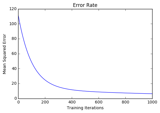
Model evaluation
After training our model through 1000 iterations with a learning rate of .0005, we finally arrive at a set of weights we can use to make predictions:
Our MSE cost dropped from 110.86 to 6.25.
References
| [1] | https://en.wikipedia.org/wiki/Linear_regression |
| [2] | http://www.holehouse.org/mlclass/04_Linear_Regression_with_multiple_variables.html |
| [3] | http://machinelearningmastery.com/simple-linear-regression-tutorial-for-machine-learning |
| [4] | http://people.duke.edu/~rnau/regintro.htm |
| [5] | https://spin.atomicobject.com/2014/06/24/gradient-descent-linear-regression |
| [6] | https://www.analyticsvidhya.com/blog/2015/08/common-machine-learning-algorithms |